The Middle Layer: Why Compilers Generate Intermediate Code

This article is Part 5 of the Compiler Design series. Part 1 · Part 2 — Lexical Analysis · Part 3 — Syntax Analysis · Part 4 — Semantic Analysis

By the end of semantic analysis, the compiler has a fully type-annotated AST. The programme has been checked for every error the front end can detect. Now comes the pivotal question: how do you turn a tree into machine instructions?

The answer is: you don’t go directly. You generate an intermediate representation first.

Why Not Go Straight to Machine Code?

Compiling directly from AST to machine code is theoretically possible, but it creates serious problems in practice:

The M × N problem. Suppose you have M source languages (C, C++, Rust, Go) and N target architectures (x86, ARM, RISC-V, WebAssembly). A direct approach requires M × N compilers. An IR approach requires M front ends + N back ends, with the IR as the shared contract between them. LLVM is built exactly on this model — dozens of languages compile to LLVM IR, and from there to any supported architecture.

Optimisation is harder on ASTs. Trees are the right structure for parsing and type-checking, but they’re awkward for the kind of transformations an optimiser needs to apply. A flat, linear IR is much easier to analyse — data-flow analysis, loop detection, and register allocation all work on linear sequences, not trees.

Machine code is target-specific. Writing machine code requires knowing register counts, instruction sets, and calling conventions for a specific CPU. Mixing that knowledge into the tree-walking stage creates a tightly coupled, unmaintainable mess.

The IR decouples these concerns: the front end produces IR, the optimiser improves it, and the back end translates it to the target architecture — each stage focused on one job.

What is Intermediate Representation?

An Intermediate Representation (IR) is a data structure that sits between the AST and machine code. A good IR is:

• Simple — each instruction does one well-defined thing
• Explicit — every operation and type is spelled out; no implicit conversions
• Machine-independent — no registers, no calling conventions, no platform assumptions
• Easy to analyse — data dependencies are obvious; optimisations are straightforward to apply

The compiler’s IR generator walks the annotated AST and produces IR instructions, one or a few per AST node.

Three-Address Code

The most widely studied IR form is three-address code (TAC). Each instruction has the form:

result = operand₁  operator  operand₂

At most three addresses: a destination and up to two source operands. The name “three-address” refers to the fact that each instruction can name up to three locations — a result and two inputs — rather than the one address of a stack machine or the two of a two-address accumulator architecture.

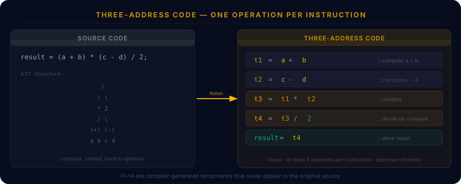
For the source expression result = (a + b) * (c - d) / 2, the TAC is:

t1 = a + b
t2 = c - d
t3 = t1 * t2
t4 = t3 / 2
result = t4

Each t1, t2, etc. is a temporary variable — a compiler-generated name that holds an intermediate value. Temporaries never appear in the original source; they exist only in the IR, and the back end will eventually assign them to machine registers.

Why TAC is Optimiser-Friendly

The decomposition into single-operation instructions makes data dependencies explicit. From the TAC above, an optimiser can immediately see:

• t1 and t2 are independent — they could be computed in parallel
• t3 depends on both t1 and t2
• If a + b appears elsewhere in the programme, t1 could be reused (common subexpression elimination)
• If 2 is a power of two, / 2 can be replaced with a right-shift (strength reduction)

None of these observations are easy to make from a nested AST.

Where IR Sits in the Pipeline

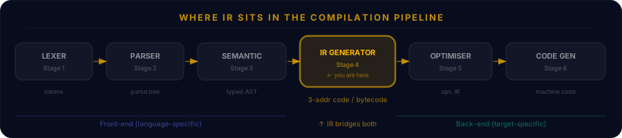
The IR is the seam between the front end and the back end:

• Front end (Stages 1–3): language-specific. Understands C syntax, Python semantics, Rust ownership rules. Produces IR.
• IR: the common language. Knows nothing about the source language or the target machine.
• Back end (Stages 5–6): machine-specific. Understands x86 instruction encoding, ARM calling conventions. Consumes IR.

This separation is the reason GCC and LLVM can compile multiple languages to multiple targets without writing M × N specialised compilers.

Other IR Forms

Three-address code is not the only option. Compilers use several IR forms depending on what analyses they need to perform:

Static Single Assignment (SSA)

In SSA form, every variable is assigned exactly once. When a variable might have been set by one of several paths (e.g., before and inside an if-else), SSA introduces a special φ (phi) node to merge the possibilities. SSA makes data-flow analysis dramatically simpler and is used in LLVM IR, the JVM bytecode verifier, and GCC’s middle-end.

Control Flow Graph (CFG)

A CFG represents the programme as a graph of basic blocks — straight-line sequences of instructions with a single entry and single exit. Edges represent possible transfers of control (jumps, branches). The CFG is the natural structure for loop detection, liveness analysis, and register allocation.

Bytecode

Java’s .class files, Python’s .pyc files, and WebAssembly are all bytecode — a compact, stack-based IR designed to be executed by a virtual machine or JIT-compiled at load time. Bytecode prioritises portability and small file size over optimisability.

A Concrete Example: Compiling a Function

Given this C function:

int square_sum(int a, int b) {
    int s = a + b;
    return s * s;
}

A three-address code IR for it might look like:

square_sum:
  t1 = a + b
  s  = t1
  t2 = s * s
  return t2

Notice:

• Parameter names a and b are used directly (the back end will assign them to registers or stack slots)
• Each operation is one instruction
• The function’s structure is preserved; return is an explicit IR instruction

The optimiser will immediately spot that s = t1 is unnecessary — it can substitute t1 directly wherever s appears, eliminating the extra assignment.

What Comes Next

The IR is handed to the optimiser — Stage 5. The optimiser’s job is to transform the IR to produce faster or smaller code, applying transformations like constant folding, dead code elimination, and loop optimisation — all without changing the programme’s observable behaviour. That’s the subject of the next article in this series.