Doing More With Less: How Compilers Optimise Your Code

This article is Part 6 of the Compiler Design series. Part 1 · Part 2 · Part 3 · Part 4 · Part 5

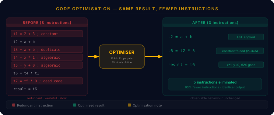
By this point in the pipeline, the compiler has a valid IR for the programme — correct, but not necessarily efficient. The optimiser is the stage that asks: can we say the same thing with fewer instructions?

The word “optimisation” is a slight misnomer. The compiler doesn’t produce optimal code in any mathematical sense — that problem is generally undecidable. It produces improved code: faster, smaller, or both, within a bounded compilation time.

The single inviolable constraint: the optimised programme must produce identical observable output to the unoptimised one. The optimiser can change how the programme computes its answer; it cannot change the answer.

Where Optimisation Happens

Optimisation is applied to the IR, not to source code or machine code. This is deliberate: the IR is the ideal level of abstraction.

• High enough that the compiler understands intent (this is an addition, this is a loop)
• Low enough that data dependencies between instructions are explicit
• Machine-independent, so optimisations written once apply to every target

Local Optimisations

Local optimisations work within a single basic block — a straight-line sequence of instructions with no branches. They’re the simplest and fastest to apply.

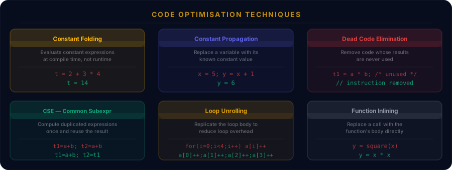
Constant Folding

If both operands of an expression are known constants at compile time, compute the result immediately:

; Before
t1 = 60 * 60 * 24      ; computes to 86400

; After
t1 = 86400             ; constant folded at compile time

There is no reason to emit a multiplication instruction when the result is already known. The programme will execute the multiplication zero times instead of once every time this code runs.

Constant Propagation

After a constant assignment, substitute the constant wherever the variable is used:

; Before
x = 5
y = x + 3

; After
y = 8              ; x replaced with 5, then folded

Constant propagation often triggers further constant folding — the two optimisations interact and amplify each other.

Algebraic Simplification

Apply mathematical identities to reduce instructions:

t = x * 1        → t = x          ; multiply by 1 is identity
t = x + 0        → t = x          ; add 0 is identity
t = x * 0        → t = 0          ; multiply by 0 is zero
t = x * 2        → t = x + x      ; or: t = x << 1  (shift is cheaper)

The last example — replacing multiplication by a power of two with a left shift — is called strength reduction: replacing an expensive operation with a cheaper one that produces the same result.

Common Subexpression Elimination (CSE)

If the same expression is computed more than once and its operands haven’t changed in between, compute it once and reuse the result:

; Before
t1 = a + b
t2 = a + b     ; identical computation

; After
t1 = a + b
t2 = t1        ; reuse t1 instead of recomputing

CSE can cascade significantly — a large expression tree may share dozens of sub-computations.

Dead Code Elimination

Code whose result is never used — because the variable is never read, or because the code is unreachable — is simply removed:

; Before
t1 = x * y     ; t1 is never read after this
t2 = a + b
result = t2

; After
t2 = a + b     ; t1 computation removed entirely
result = t2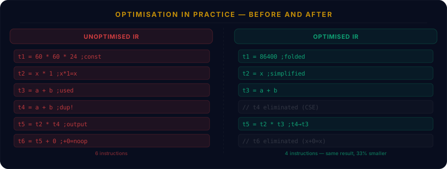

Loop Optimisations

Loops are where programmes spend the majority of their runtime. A loop body that executes a million times will amplify any inefficiency a millionfold. Loop optimisations are therefore among the highest-impact transformations a compiler can apply.

Loop-Invariant Code Motion (LICM)

If a computation inside a loop produces the same result on every iteration, move it outside the loop:

// Before
for (int i = 0; i < n; i++) {
    x = a * b;       // a and b don't change; why compute this n times?
    arr[i] = x + i;
}

// After
x = a * b;           // hoisted: computed once before the loop
for (int i = 0; i < n; i++) {
    arr[i] = x + i;
}

This turns O(n) multiplications into O(1).

Loop Unrolling

Reduce loop overhead (incrementing the counter, checking the condition, branching back) by duplicating the body:

// Before
for (int i = 0; i < 4; i++) arr[i] *= 2;

// After (unrolled by 4)
arr[0] *= 2;
arr[1] *= 2;
arr[2] *= 2;
arr[3] *= 2;

When the trip count is not known at compile time, partial unrolling (factor of 2, 4, or 8) is applied with a tail to handle remaining iterations. Unrolled loops also allow the CPU’s superscalar execution units to work in parallel on multiple independent operations.

Induction Variable Simplification

An induction variable is one that changes by a fixed amount each iteration. If a more expensive expression is derived from it, replace the expression with a simpler update:

// Before
for (int i = 0; i < n; i++) {
    p = &arr[i * 4];   // multiplication on every iteration
}

// After
for (int* p = arr; p < arr + n * 4; p += 4) {
    // p incremented by 4 (add only) each time
}

Interprocedural Optimisations

These optimisations cross function boundaries and require the compiler to analyse multiple functions together.

Function Inlining

Replace a function call with the function’s body at the call site:

// Before
int square(int x) { return x * x; }
int y = square(a + b);

// After inlining
int t = a + b;
int y = t * t;   // call eliminated entirely

Inlining removes the overhead of the call (saving and restoring registers, stack frame setup) and — crucially — exposes the body of the function to the caller’s optimiser, enabling further local optimisations that wouldn’t be visible across the function boundary.

Inlining is a trade-off: it speeds up the call but increases code size. Compilers apply heuristics (function size, call frequency, whether it’s in a hot loop) to decide when inlining is beneficial.

Dead Function Elimination

Functions that are never called are removed from the output. This is especially valuable in languages with large standard libraries — only the functions actually used end up in the final binary.

How Optimisations Interact

Optimisations don’t work in isolation — they enable each other. Constant propagation creates more opportunities for constant folding; inlining exposes code to CSE; dead code elimination cleans up after constant propagation removes all uses of a variable.

For this reason, optimisers run multiple passes over the IR, repeatedly applying transformations until no further improvements can be found (or a pass budget is exhausted).

Optimisation Levels

Real compilers expose optimisation as a dial rather than a switch. GCC and Clang define four main levels:

The trade-off is compile time vs. runtime speed. -O0 compiles in seconds; -O3 on a large C++ codebase can take minutes.

What the Optimiser Cannot Do

Some things are off-limits:

• Removing visible side effects. If a function writes to a file or sends a network packet, the compiler cannot eliminate that call even if its return value is unused.
• Reordering observable operations. The memory model of the language constrains what reorderings are legal, especially in concurrent code.
• Changing floating-point behaviour. Due to rounding rules, (a + b) + c is not always equal to a + (b + c) in floating-point arithmetic. Most compilers won’t reassociate floating-point operations without explicit permission (-ffast-math in GCC/Clang).

These constraints are what the phrase “without changing observable behaviour” actually means in practice.

What Comes Next

After optimisation, the IR is handed to the machine code generator — the final stage of compilation. The code generator maps the optimised IR onto the specific instruction set of the target machine: assigning variables to registers, selecting instructions, handling calling conventions, and producing the binary output that the CPU can actually execute.

That final stage — and with it, the full picture of how source code becomes a running programme — is the subject of the next article in this series.